Accelerating Quantum Kernel Computation with Joblib

How to unleash the full power of your CPU cores to expedite quantum kernel computations.

One of the areas where quantum computers could offer an advantage in the future is in computing specialized kernel functions that underlie Support Vector Machines (SVMs). However, simulating these quantum kernels on classical hardware can be extremely time-consuming, especially as the dataset size grows.

In this blog post, we’ll explore the complexity of computing quantum kernel matrices for large datasets and demonstrate how using joblib, a Python library for parallelizing tasks, can significantly speed up this process. We’ll walk through code snippets that:

1. Define and compute a quantum kernel without parallelization.

2. Introduce parallelization using joblib.

3. Show the performance gains and discuss the results.

As you probably know already, a quantum kernel encodes classical data into quantum states and measures an overlap (or fidelity) between these states. When used in SVMs, these kernels can potentially separate data in complex, high-dimensional feature spaces with fewer resources than their classical counterparts—at least in theory. However, simulating quantum kernels on classical machines involves running a quantum circuit simulation for each pair of training points, leading to a computational complexity that scales poorly with dataset size.

For a dataset with N samples, computing a full kernel matrix requires N² circuit evaluations. Each evaluation is expensive, and as N grows, the precomputation time can become a major bottleneck. This is where parallelization comes in.

joblib provides a simple, high-level interface for parallelizing Python code across multiple cores of your CPU. By distributing the computation of each row (or chunk) of the kernel matrix among different workers, we can significantly reduce the total computation time.

import time
import numpy as np
from sklearn.datasets import make_classification
from sklearn.model_selection import train_test_split
from sklearn.svm import SVC
import pennylane as qml

# Create a synthetic dataset
X, y = make_classification(n_samples=200, n_features=4, n_informative=2, 
                           n_redundant=0, n_classes=2, random_state=42)
X_train, X_test, y_train, y_test = train_test_split(X, y, test_size=0.2, random_state=42)

# Setup the quantum device and number of qubits
n_qubits = X_train.shape[1]
dev = qml.device("default.qubit", wires=n_qubits, shots=None)

def feature_map(x):
    for i, val in enumerate(x):
        qml.RX(val, wires=i)

@qml.qnode(dev)
def kernel_circuit(x1, x2):
    feature_map(x1)
    qml.adjoint(feature_map)(x2)
    return qml.expval(qml.Projector([0]*n_qubits, wires=range(n_qubits)))

def compute_kernel_row(i, X1, X2):
    return [kernel_circuit(X1[i], X2[j]) for j in range(X2.shape[0])]

def quantum_kernel_serial(X1, X2):
    m1 = X1.shape[0]
    K = np.zeros((m1, X2.shape[0]))
    for i in range(m1):
        K[i, :] = compute_kernel_row(i, X1, X2)
    return K

Purpose of the code:

• Generate a synthetic dataset.

• Define a quantum kernel using PennyLane.

• Implement a function to compute the kernel matrix using a serial (non-parallelized) approach.

How it works:

• We use scikit-learn to create a synthetic binary classification dataset.

• We define a feature_map that encodes classical data into quantum states by applying rotations.

• We create a QNode (kernel_circuit) that returns the fidelity between two encoded states.

• Finally, we implement quantum_kernel_serial to compute the entire kernel matrix by iterating through all sample pairs.

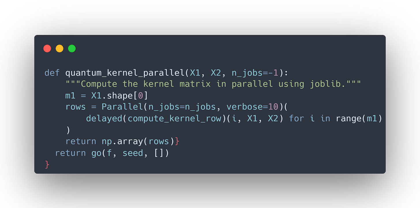
from joblib import Parallel, delayed

def quantum_kernel_parallel(X1, X2, n_jobs=-1):
    m1 = X1.shape[0]
    rows = Parallel(n_jobs=n_jobs, verbose=10)(
        delayed(compute_kernel_row)(i, X1, X2) for i in range(m1)
    )
    return np.array(rows)

Purpose of the code:

• Use joblib to parallelize the kernel computation.

• Define a quantum_kernel_parallel function that computes the kernel matrix with multiple workers.

How it works:

• We import joblib.Parallel and delayed.

• Instead of computing each row of the kernel matrix in a for-loop, we submit these tasks to the Parallel backend.

• Setting n_jobs=-1 ensures that all available CPU cores are utilized. In this case 16 cores.

# Compare computation times
start_time = time.time()
K_train_serial = quantum_kernel_serial(X_train, X_train)
K_test_serial = quantum_kernel_serial(X_test, X_train)
no_parallel_time = time.time() - start_time

start_time = time.time()
K_train_parallel = quantum_kernel_parallel(X_train, X_train, n_jobs=-1)
K_test_parallel = quantum_kernel_parallel(X_test, X_train, n_jobs=-1)
parallel_time = time.time() - start_time

print("=== Comparison of Precomputation Times ===")
print(f"No parallelization: {no_parallel_time:.4f} seconds")
print(f"Parallelization   : {parallel_time:.4f} seconds\n")

# Check if kernels match
assert np.allclose(K_train_serial, K_train_parallel, atol=1e-6)
assert np.allclose(K_test_serial, K_test_parallel, atol=1e-6)

# Train SVC to confirm correctness
start_time = time.time()
qsvc = SVC(kernel='precomputed')
qsvc.fit(K_train_parallel, y_train)
acc = qsvc.score(K_test_parallel, y_test)
end_time = time.time()

Purpose of the code:

• Compute the kernel matrices both serially and in parallel.

• Compare the timings and confirm that the kernels are equivalent.

• Train an SVC on the parallel-computed kernel to ensure correctness.

How it works:

• We measure the time for the serial computation.

• Then we measure the time for the parallel computation.

• We assert that both results are approximately the same (to ensure no numerical errors).

• Finally, we train an SVC using the precomputed kernel and show that accuracy remains the same.

Results

For a dataset of 200 samples and a 4-qubit quantum feature map, we observed the following performance:

=== Comparison of Precomputation Times ===
No parallelization: 35.9270 seconds
Parallelization   : 8.4191 seconds

Here we see a substantial speedup:

• Without parallelization: ~35.9 seconds

• With parallelization: ~8.4 seconds

That’s more than a 4x improvement in performance simply by utilizing all available cores!