Dimensionality Reduction for Quantum Machine Learning: Integrating LDA and K-Means

This article provides an illustration of how a dataset could be effectively reduced to execute QML that requires a low range of dimensions.

In Quantum Machine Learning (QML), the preparation of data is a crucial step that often determines the effectiveness and efficiency of the algorithms used. One of the key challenges in this process is dimensionality reduction, which involves transforming high-dimensional data into a lower-dimensional space. This is particularly important in quantum computing, where managing complexity and computational load is paramount. In this context, we will explore the integration of Linear Discriminant Analysis (LDA) and K-means clustering as methods for effective dimensionality reduction, preparing the data optimally for subsequent processing with QML algorithms.

The Role of LDA and K-means

Linear Discriminant Analysis (LDA)

LDA is a technique used to find the linear combinations of features that best separate two or more classes of objects or events. The resulting combination can be used as a linear classifier or for dimensionality reduction before later classification. In the context of QML, LDA serves as a pre-processing step that simplifies the data, reducing the number of features to a manageable size for the quantum algorithms, while preserving as much class discriminatory information as possible.

K-means Clustering

K-means is a widely-used method in unsupervised machine learning for partitioning data into K distinct clusters based on feature similarities. In the process of preparing data for QML, K-means can be employed to group features or data points into clusters. This clustering can reveal hidden patterns in the data, assisting in identifying the most relevant features or reducing the dimensionality of the dataset. By doing so, it helps in mitigating the curse of dimensionality often faced in quantum computing.

Preparing the Environment

Importing Libraries

import numpy as np
import pandas as pd
import matplotlib.pyplot as plt
import sklearn as sklearn
from sklearn.model_selection import train_test_split
from sklearn.preprocessing import StandardScaler, MinMaxScaler, normalize
from sklearn.discriminant_analysis import LinearDiscriminant Analysis as LDA
from sklearn.cluster import KMeans

This code block imports the necessary libraries and sets up the environment. We use numpy and pandas for data manipulation, matplotlib for visualization, and various sklearn modules for machine learning tasks.

Loading and Preprocessing the Data

Loading the Dataset

df = pd.read_csv('yourdataset.csv')
df = df.sample(1000, random_state=42)

The dataset is loaded and a sample of 1000 entries is selected for analysis to manage the computational load (especially in quantum machine learning challenges).

Preparing the Data

X = df.drop(['target'], axis="columns")
y = df['target']
X_train, X_test, y_train, y_test = train_test_split(X, y, test_size=0.20, random_state=42)

The features (X) and target variable (y) are separated, and the data is split into training and testing sets.

Handling Constant Columns

constant_columns = X_train.columns[X_train.nunique() == 1]
X_train = X_train.drop(columns=constant_columns)
X_test = X_test.drop(columns=constant_columns)

Constant columns, which do not vary and hence provide no useful information for modeling, are identified and removed.

Calculating Feature Correlations

correlations = X_train.corrwith(y_train)

This calculates the correlation of each feature with the target variable.

Visualizing Correlations

correlations.plot(kind='bar', figsize=(10,7))
plt.title('Correlation with target variable')
plt.xlabel('Features')
plt.ylabel('Correlation coefficient')
plt.show()

This code visualizes the correlations as a bar plot, providing insight into how each feature relates to the target variable.

Feature Processing and Clustering

K-Means Clustering of Features

num_dimensions = 2
correlations_reshaped = np.reshape(correlations.values, (-1, 1))
kmeans = KMeans(n_clusters=num_dimensions, random_state=0).fit(correlations_reshaped)
clusters = kmeans.labels_
groups = [np.where(clusters == i)[0] for i in range(num_dimensions)]

Here, we reshape the correlations and apply K-means clustering to group features based on their correlation with the target variable and the number of pre-defined dimensions.

Visualizing Feature Clusters

for i in range(num_dimensions):
    plt.scatter(groups[i], correlations[groups[i]], label=f'Cluster {i}')
plt.xlabel('Features')
plt.ylabel('Correlation coefficient')
plt.title('Cluster Assignments based on Correlation')
plt.legend()
plt.show()

This block of code visualizes the clusters, showing how features are grouped based on their correlation coefficients.

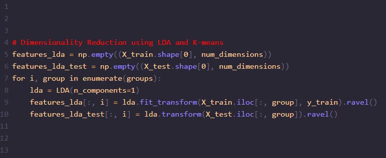
Creating New Features with LDA

features_lda = np.empty((X_train.shape[0], num_dimensions))
features_lda_test = np.empty((X_test.shape[0], num_dimensions))
for i, group in enumerate(groups):
    lda = LDA(n_components=1)
    features_lda[:, i] = lda.fit_transform(X_train.iloc[:, group], y_train).ravel()
    features_lda_test[:, i] = lda.transform(X_test.iloc[:, group]).ravel()

LDA is applied to each group of features to create new, reduced-dimensionality features that are more suitable for classification tasks.

Normalizing Data

minmax_scaler = MinMaxScaler().fit(features_lda)
X_train_qml = minmax_scaler.transform(features_lda)
X_test_qml = minmax_scaler.transform(features_lda_test)

Here we are using MinMaxScaler to normalize the output, but several techniques can be used that are more suitable for the QML model that you will apply later on.

By preparing the data with LDA and K-means for dimensionality reduction and then normalizing it with MinMaxScaler, we create an optimal environment for models like QSVC to perform effectively enough in a quantum computing framework. It is important to notice, that this is just an initial step and will not secure good results since this will depend on the dataset, feature maps, model selected, parameters and several other adjustments.