D-Wave's New Chip and How to Use it

Even if it is still a prototype.

Some of you may have already heard the news about D-Wave’s new chip. if not, here is the link:

1200 qubit chip

Wait, but didn’t D-Wave already manufacture chips in the range of thousands of qubits? Yes, but these are better.

They do mention that this chip has some beautiful new features:

• Qubit connectivity: increased from 15 to 20-way connectivity to enable solutions to larger problems

• Energy scale: increased by more than 40% to deliver higher-quality solutions

• Qubit coherence time: doubled, which will drive faster time-to-solution

Well, let’s try that out. As you know, D-Wave provides access through their Leap platform.

https://cloud.dwavesys.com/leap/

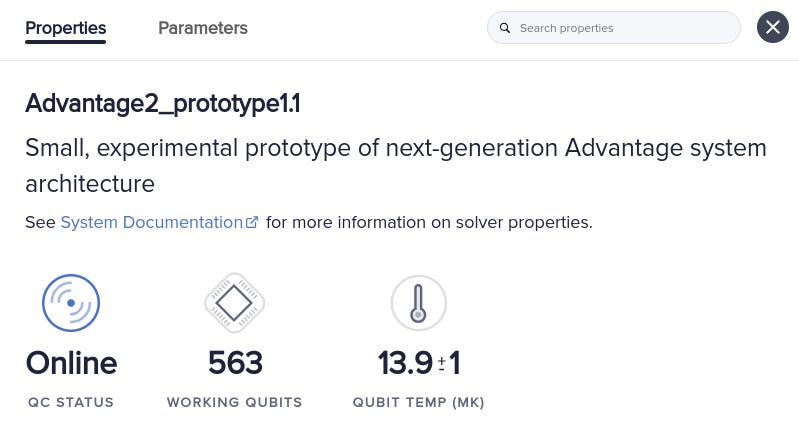
And if you log in, you will see a new system has been added

It is not as big as advertised but it does look better than his old predecessors

If you would like to give it a test, here are some things you should do beforehand.

Setting things up

You will need to retrieve and copy the API from the Leap platform

And then open your preferred Python editor. There are some libraries you might need, including:

pip install dwave-system dimod pyqubo

Won’t put the versions there but the ones that I am using for this code are:

dimod==0.12.3

dwave-system==1.18.0

pyqubo==1.4.0

Once you have those, you will need a problem to be solved. You could either select a random Ising type of problem or you can take one from some of our previous posts, like the one about Quantum Feature Selection, for example.

Let’s assume you have your problem selected. You know that QUBO, Ising, or BQM problems can be translated thanks to dimod functionalities: https://docs.ocean.dwavesys.com/en/stable/docs_dimod/reference/generated/dimod.utilities.qubo_to_ising.html

Assuming you have your linear (h) and quadratic coefficients for the Ising model example, you can build the Binary Quadratic Model (BQM) like

import dimod

bqm = dimod.BQM.from_ising(h, J)

Getting access to the QPU

It could not be easier; simply use your token and look for the available QPUs.

from dwave.cloud import Client

client = Client.from_config(token="<YOUR TOKEN>")
client.get_solvers()

You will see that those names correspond to the same ones on the Leap platform. Simply select the Advantage2 prototype.

qpu = client.get_solver(name="Advantage2_prototype1.1")

And simply run your problem on it…

sampler = qpu.sample_bqm(bqm, label="QFS")

Well, most likely it will show something like this…

ProblemStructureError: Problem graph incompatible with Advantage2_prototype1.1 solver

Mapping your problem to the QPU

As you may know, Binary Quadratic Model variables need to be mapped to the architecture of the chip. Even though this one counts with more connections, there is still some embedding that needs to be done. My BQM has 13 variables, but all to all connected, which will require linking some of the qubits of the chip together so they represent the same variable. This is what D-Wave calls chain management

https://docs.dwavesys.com/docs/latest/handbook_embedding.html#chain-management

Do not confuse it with management chain; that is a different story.

Our QPU edges can be requested as follows:

>>> qpu.edges

{(539, 543),
 (476, 78),
 (285, 281),
 (84, 377),
 (142, 498),
 (346, 148),
...

And our problem has quadratic terms as follows:

>>> bqm.quadratic

{('x[8]', 'x[7]'): 0.25347981366005845, ('x[6]', 'x[7]'): 0.2653609023143667, ('x[6]', 'x[8]'): ...

Then, we need to find an embedding that maps those together.

from minorminer import find_embedding

embedding = find_embedding(bqm.quadratic, qpu.edges)
embedding

Voilà!

{'x[8]': [202, 203], 'x[7]': [210, 467], 'x[6]': [491, 198], 'x[5]': [494, 214], 'x[9]': [499, 230], 'x[4]': [483, 246], 'x[3]': [206], 'x[11]': [507, 238], 'x[10]': [510, 222], 'x[2]': [451], 'x[0]': [455, 454], 'x[12]': [218, 459], 'x[1]': [250, 475]}

It represents that for our variable x[8] for example, it will be mapped to the 202 and 203 qubits on the chip to enable its connection to the rest of the variables. In that embedding, we can look for a translation of our problem so that the QPU will understand what qubits we need to use and the value weight (the quadratic term J) it should be used for each of them.

from dwave.embedding import embed_bqm, EmbeddedStructure

e_struct = EmbeddedStructure(qpu.edges, embedding)
e_bqm = embed_bqm(bqm, e_struct)

That new BQM problem is the one we can run on our device and check when it’s done.

sampler = qpu.sample_bqm(e_bqm, label="QFS")
sampler.done()

Then retrieve the results.

result = sampler.result()
results

{'solutions': [[0, 0, 0, 0, 0, 0, 0, 0, 0, 0, 0, 0, 0, 0, 0, 0, 0, 0, 0, 0, 0, 0, 0, 0, 0,

...

507, 510], 'num_variables': 576, 'offset': 29.285343671784812, 'problem_type': 'ising'}

Oh my! 576 variables? Don’t panic.

Translating back

Some of them are active variables, and others are simply the remaining qubits of the chip. You can retrieve from the set of solutions…

first = result['solutions'][0]

The energies and active variables

vars = result['active_variables']
e = result['energies']

And get just the -1s and 1s of your Ising problem.

solution = []
for v in vars:
    solution.append(first[v])
solution

It will still show more variables than the original ones, due to the embedding. You simply need to translate those back.

translated_solution = {}

for k in embedding:
    for var in embedding[k]:
        if k not in translated_solution:
            translated_solution[k] = [first[var]]
        else:
            translated_solution[k] += [first[var]]

And you will see the values of each qubits associated with you problem variables.

{'x[8]': [-1, -1],
 'x[7]': [-1, -1],
 'x[6]': [-1, -1],
 'x[5]': [-1, -1],
 'x[9]': [-1, -1],
 'x[4]': [-1, -1],
 'x[3]': [-1],
 'x[11]': [1, 1],
 'x[10]': [-1, -1],
 'x[2]': [-1],
 'x[0]': [-1, -1],
 'x[12]': [1, 1],
 'x[1]': [-1, -1]}

Now you are ready to tackle larger problems! Happy annealing :)